In the last article I wrote, I talked about a way to measure the competitiveness of a given IndyCar season. If you haven’t read that article, I would recommend doing so before continuing with this one. That measure was a fairly good first attempt at measuring competitiveness: it gave a good idea of the spread of the field and how dominant the champion was. Kyle Brown, a fellow IndyCar blogger who focuses on the statistics and data of the sport, left a comment on that post suggesting a different approach to measuring competitiveness that built off of what I started with. Kyle’s suggestion was to sum all of the competitiveness ratios (now referred to as CR) for a given set of the field (we looked at sums of the top-10, top-5, and top-3 drivers specifically). Then, we averaged the ratios for all drivers for each of the sets we looked at — for example, for the top-3 set, we summed second place’s CR and third place’s CR and averaged them. This leaves us with Average Competitiveness Ratio or ACR. As a reminder, an individual place’s CR is given by:
CR = (Champion’s Points – X Place’s Points)/Total Possible Points for a Driver
The advantage of this system over my original is that it takes into account how close each driver was to the champion as opposed to just the X place driver. For example, consider the following two seasons. In hypothetical season A, the top-9 drivers were all separated by one point each and the tenth driver was 200 points back from the champion. In hypothetical season B, the top-9 drivers were all separated by 20 points and and tenth driver was 200 points back from the champion. Under my original method, these seasons would both have the same competitiveness ratio for the top-10 of the field. Under the new system, season A would be considered more competitive (as it should be, because there are more drivers in the championship battle and close to each other) because it’s ACR would be less than season B’s. My original method is a good measure of thecompetitiveness in terms of the spread of the field, but ACR is a better measure of how competitive all of the drivers were in terms of the championship battle.
Once again, this process gives us a ratio for each season from 0 to 1. The former would be a perfectly competitive season (all drivers score the same number of points) and the latter would be a perfectly non-competitive season (there is one driver winning every possible point in every race and the other drivers aren’t even competing).
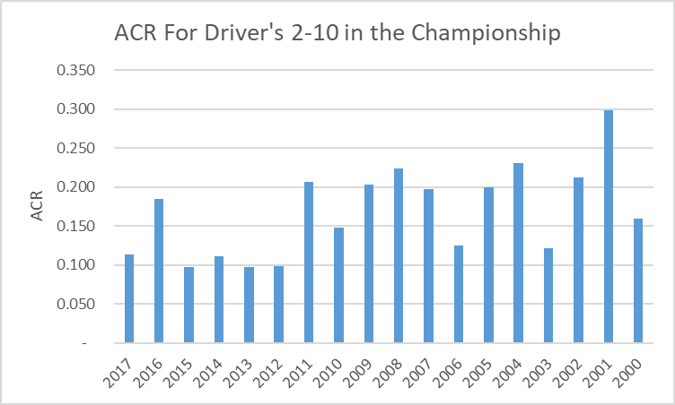
Now that we’ve got the description out of the way, we can get into the results. First, let’s look at the ACR for the top-10 drivers in the seasons 2000-17.
The 2015 and 2013 seasons both had an ACR of 0.097, making them the most competitive seasons in terms of top-10 competitiveness in our data set. For comparison, 2015 — when Juan Pablo Montoya and Scott Dixon ended up tied in the points after Sonoma — was the most competitive season by my original method. 2001 was the least competitive year as Sam Hornish Jr. won the championship 100 points clear of the field. We see the same drop off at the 2012 season that we saw the last time around, and once again, I think this could be because of the adoption of the Dallara DW-12 chassis. It seems to have made the field more competitive on the whole (or at least the top half of the field).
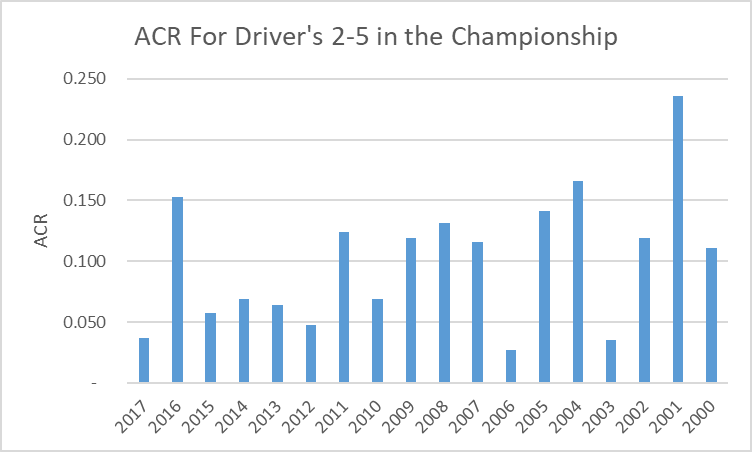
We get the following graph for the top-5 spots in the championship.
The results show us that 2006 had the most competitive top-5 championship. This season the top four places in the championship were separated by just 15 points. Hornish Jr. and Dan Wheldon were tied after the last race and the former won on a tiebreaker. Six different drivers took home race wins and nine different drivers finished on the podium.
And finally, we have the graph for the top-3.
2006 was the most competitive season for the top-3 places in the championship, for the same reasons mentioned above. 2001 was the least competitive season for the top-3, largely in part because the champion was 100 points clear of the runner up. And in 2016, Simon Pagenaud won by 127 points, making it the 2nd least competitive season in our time frame with an ACR of 0.14.
Using ACR as opposed to CR for a given place provides a more accurate measure for the competitiveness of a season. It takes into account all places within the specified range and shows how competitive the championship battle really was, which is, at the end of the day, what we all really care about. Exciting championship battles are a sign of an exciting season. I would say using ACR for the top-5 or top-10 drivers is my preferred range when looking at how competitive a season is, as that’s where most of the action on track takes place each race. I’d prefer a season with a lower top-5 or top-10 ACR over one with just a super low top-3 ACR, because that means many drivers are in the hunt, even if it means the gap to second or third isn’t incredibly low (<10 points). People could have different opinions on which method they prefer to look at of course.
Thanks again to Kyle for the great suggestion and help in compiling the data for this project.